
Привет, Хабр! На связи Рустем, IBM Senior DevOps Engineer & Integration Architect.
В этой статье я хотел бы рассказать об использовании машинного обучения в Streamlit и о том, как оно может помочь бизнес-пользователям лучше понять, как работает Data Science. В этой лабораторной работе мы будем использовать набор данных о страховых исках. Мы объединим мощь Streamlit с процессом обработки данных, состоящим из исследовательского анализа данных и оценки различных моделей. Я расскажу, как найти модель, которая не только работает с высокой точностью, но и позволяет бизнес-пользователям лучше понять, как мы получаем приемлемую модель. Наконец, мы увидим, как мы можем разделить информационную панель на разные вкладки и сделать ее более удобной для использования, когда мы хотим представить проект из области Data Science публике и сделать его пригодным для непосредственного использования.
Что мы хотим:
-
Использовать табы Streamlit
-
Задокументировать проект DS в Streamlit
-
Сделать машинное обучение понятным для бизнес-пользователей
Предварительные навыки, которые нам нужны:
-
Базовый опыт Python
-
Опыт работы с Pandas/Numpy/Seaborn
-
Базовый опыт машинного обучения
Но немного про Streamlit
Streamlit — отличный способ начать создавать информационные панели на Python. Всего за несколько строк вы можете написать свой дэшборд. Независимо от того, является ли ваш вариант использования простым или сложным, Streamlit может быть удобным способом иметь под рукой быстрое решение для панели мониторинга.
Шаг 1
Здесь мы собираемся импортировать довольно много библиотек, поскольку мы будем использовать их для нашей панели инструментов. Как и в случае с любым скриптом Python, на самом деле нет ограничений на количество библиотек, которые вы можете использовать.
cat << EOF > /tmp/test.py import numpy as np import pandas as pd import matplotlib.pyplot as plt import timeit import warnings warnings.filterwarnings("ignore") import streamlit as st import streamlit.components.v1 as components #Import classification models and metrics from sklearn.linear_model import LogisticRegression from sklearn.neighbors import KNeighborsClassifier from sklearn.svm import SVC from sklearn.ensemble import RandomForestClassifier,ExtraTreesClassifier from sklearn.model_selection import cross_val_score #Import performance metrics, imbalanced rectifiers from sklearn.metrics import confusion_matrix,classification_report,matthews_corrcoef from imblearn.over_sampling import SMOTE from imblearn.under_sampling import NearMiss np.random.seed(42) #for reproducibility since SMOTE and Near Miss use randomizations from pandas_profiling import ProfileReport from streamlit_pandas_profiling import st_profile_report EOFСамая интересная часть следующего фрагмента — это то, как мы собираемся использовать боковую панель для разделения панели инструментов на разные страницы, которые пользователь (или вы) может использовать для объяснения того, как работает панель. Как видите, мы добавили здесь страницу «О нас», поскольку она помогает объяснить, что мы здесь делаем и как работает панель инструментов.
Пожалуй, самым интересным в этом первом фрагменте является то, что мы создаем разные вкладки через боковую панель и поле выбора вместо использования виджета st.tabs. Как видите, в основном вам решать, что вы хотите делать с функциями, представленными в библиотеке Streamlit (и зависит от вашего воображения и творчества!)
cat << EOF >> /tmp/test.py st.title('Claims Prediction') df=pd.read_excel('https://github.com/Stijnvhd/Streamlit_Course/blob/main/3.%20A%20first%20ML%20example/data.xlsx?raw=true', engine='openpyxl',) #df["Exposure"] = pd.to_numeric(df["Exposure"], errors='coerce') app_mode = st.sidebar.selectbox('Mode', ['About', 'EDA', 'Analysis']) EOFЭто то, что мы создали до сих пор (хотя кажется, что это много, не удивляйтесь, если вы не увидите многого!).
Вы можете запустить панель управления, выполнив:
streamlit run /tmp/test.py --server.port 80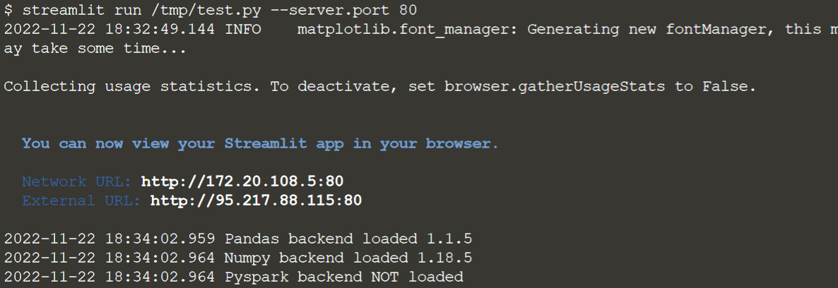

Шаг 2
Первые страницы нашего Дашборда
Как вы можете видеть в приведенном ниже фрагменте, мы сначала определяем, над какой страницей мы работаем. Еще один новый аспект, который вы видите здесь, заключается в том, что мы также добавили некоторую информацию о стилях, которая может помочь вам в дальнейшем определить, как вы хотите, чтобы панель управления выглядела. В этом случае мы добавили информацию о том, как должна выглядеть боковая панель, и информацию о том, как должен выглядеть наш Дэшборд.
Если предыдущий дэшборд все еще работает, нажмите Ctrl + C в терминале.
cat << EOF >> /tmp/test.py if app_mode == "About": st.markdown('Claims Prediction Example') st.markdown( """ <style> [data-testid="stSidebar"][aria-expanded="true"] > div:first-child{ width: 350px } [data-testid="stSidebar"][aria-expanded="false"] > div:first-child{ width: 350px margin-left: -350px } </style> """, unsafe_allow_html=True, ) st.markdown('') st.markdown('This dashboard allows you to follow the claims prediction example. It can help you to understand how we can focus on claims and in this way develop proper pricing for insurance products.') EOFСтраница About, которую мы здесь определяем, выглядит следующим образом:

Следующая страница предлагает нам некоторый исследовательский анализ набора данных. Как видите, мы добавили подзаголовок, а также описание того, как можно использовать панель управления. В зависимости от выбора, сделанного пользователем, будет отображаться различная информация в наборе данных. Как видите, мы можем без проблем вкладывать различные операторы if и связанные с ними функции:
cat << EOF >> /tmp/test.py elif app_mode == 'EDA': st.sidebar.subheader(' Quick Explore') st.markdown("Tick the box on the side panel to explore the dataset.") if st.sidebar.checkbox('Basic Info'): if st.sidebar.checkbox("Show Columns"): st.subheader('Show Columns List') all_columns = df.columns.to_list() st.write(all_columns) if st.sidebar.checkbox('Statistical Description'): st.subheader('Statistical Data Description') st.write(df.describe()) if st.sidebar.checkbox('Missing Values?'): st.subheader('Missing values') st.write(df.isnull().sum()) EOFПрежде чем пытаться запустить код, нажмите Ctrl + C, чтобы остановить запуск текущий дэшборд в вашем терминале.
Вы можете запустить панель управления, выполнив
streamlit run /tmp/test.py --server.port 80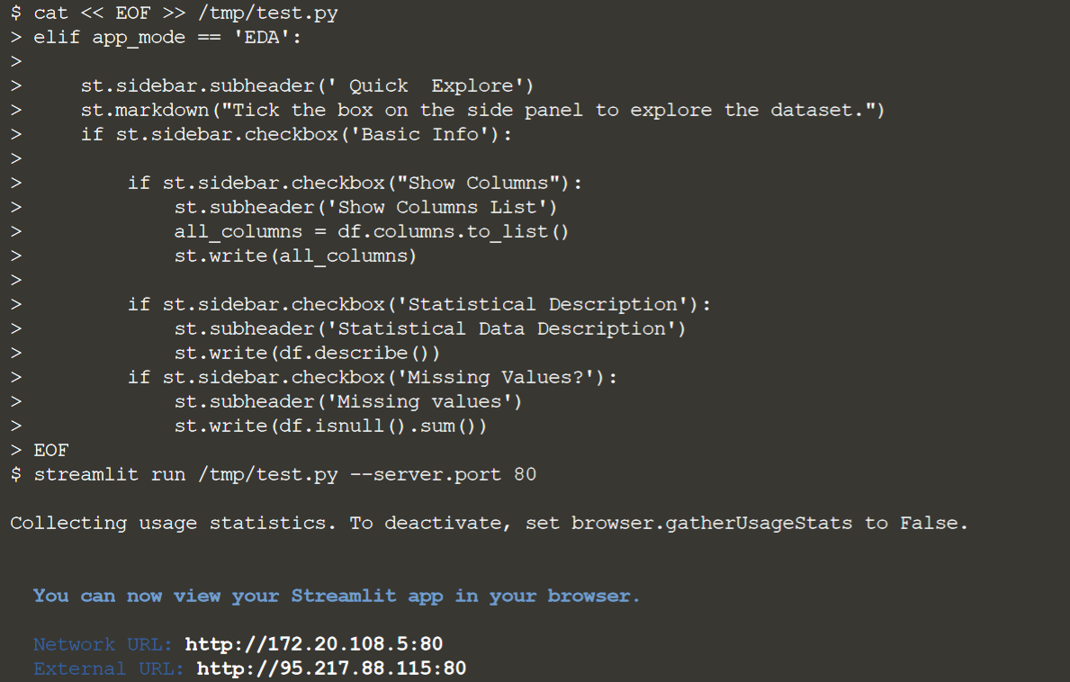
Эта часть решения будет выглядеть следующим образом:

Шаг 3. Время машинного обучения
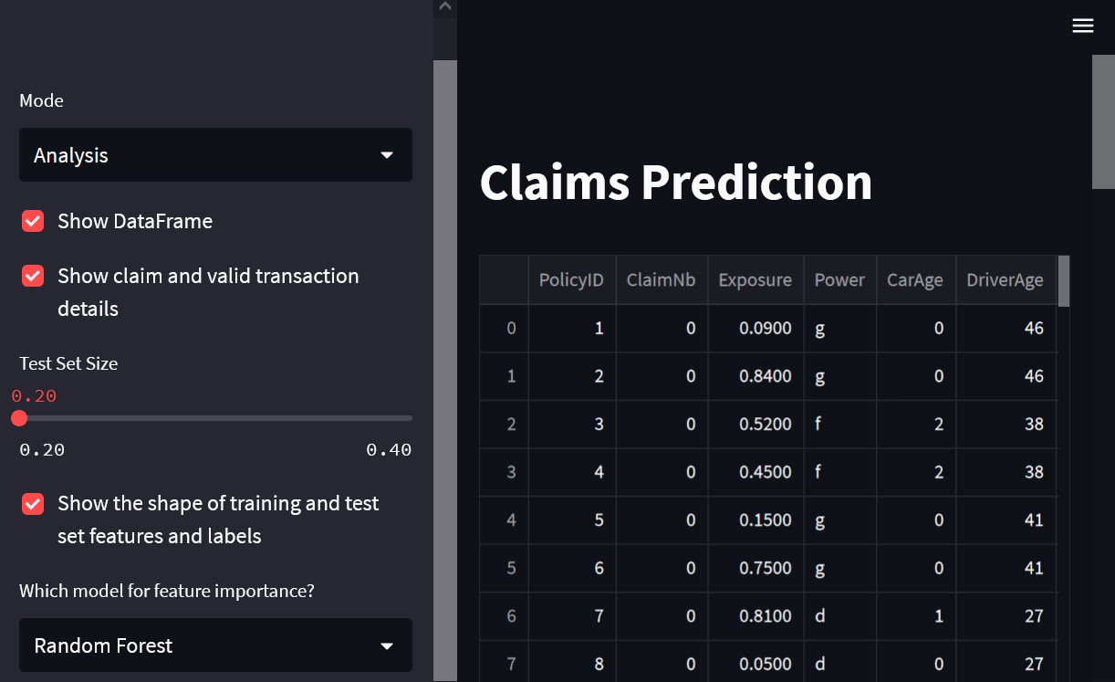
Первая часть приведенного ниже кода позволяет пользователю получить окончательный вид набора данных и некоторую ключевую информацию о том, как выглядит набор данных:
cat << EOF >> /tmp/test.py elif app_mode == "Analysis": # Print shape and description of the data st.set_option('deprecation.showPyplotGlobalUse', False) if st.sidebar.checkbox('Show DataFrame'): st.write(df.head(100)) st.write('Shape of the dataframe: ',df.shape) st.write('Data description: \n',df.describe()) # Print valid and fraud transactions fraud=df[df.ClaimNb==1] valid=df[df.ClaimNb==0] outlier_percentage=(df.ClaimNb.value_counts()[1]/df.ClaimNb.value_counts()[0])*100 if st.sidebar.checkbox('Show claim and valid transaction details'): st.write('Claim cases are: %.3f%%'%outlier_percentage) st.write('Claim Cases: ',len(fraud)) st.write('Valid Cases: ',len(valid)) EOFСледующий фрагмент состоит из некоторых ключевых шагов, которые вы обычно выполняете при работе над проектом машинного обучения. Выбираем независимые и зависимые переменные. Однако в этом случае мы позволяем пользователю выбирать размер набора тестов! Затем мы выполняем разделение набора данных и позволяем пользователю проверять функции и метки обучающего и тестового наборов.
cat << EOF >> /tmp/test.py #Obtaining X (features) and y (labels) df=df.drop(['PolicyID'], axis=1) df=df.drop(['Power'], axis=1) df=df.drop(['Brand'], axis=1) df=df.drop(['Gas'], axis=1) df=df.drop(['Region'], axis=1) df=df.dropna() X=df.drop(['ClaimNb'], axis=1) y=df.ClaimNb # Split the data into training and testing sets from sklearn.model_selection import train_test_split size = st.sidebar.slider('Test Set Size', min_value=0.2, max_value=0.4) X_train, X_test, y_train, y_test = train_test_split(X, y, test_size = size, random_state = 42) #Print shape of train and test sets if st.sidebar.checkbox('Show the shape of training and test set features and labels'): st.write('X_train: ',X_train.shape) st.write('y_train: ',y_train.shape) st.write('X_test: ',X_test.shape) st.write('y_test: ',y_test.shape) EOFЗдесь мы импортируем еще несколько моделей, которые хотим использовать, и определяем, как мы хотим использовать функции в нашей панели инструментов (дэшборде).
cat << EOF >> /tmp/test.py #Feature selection through feature importance @st.cache def feature_sort(model,X_train,y_train): #feature selection mod=model # fit the model mod.fit(X_train, y_train) # get importance imp = mod.feature_importances_ return imp #Classifiers for feature importance clf=['Extra Trees','Random Forest'] mod_feature = st.sidebar.selectbox('Which model for feature importance?', clf) start_time = timeit.default_timer() if mod_feature=='Extra Trees': model=etree importance=feature_sort(model,X_train,y_train) elif mod_feature=='Random Forest': model=rforest importance=feature_sort(model,X_train,y_train) elapsed = timeit.default_timer() - start_time st.write('Execution Time for feature selection: %.2f minutes'%(elapsed/60)) EOFОкончательный фрагмент кода выглядит довольно обширным и, возможно, пугающим, но если вы посмотрите внимательнее, вы увидите много повторений, основанных на выборе, сделанном пользователем, и на том, какую модель он хочет использовать для обучения и фактического использования модели.
В зависимости от выбора модели вы можете добавить алгоритм для определения наиболее важных функций, которые можно использовать в выбранной вами модели.
cat << EOF >> /tmp/test.py #Plot of feature importance if st.sidebar.checkbox('Show plot of feature importance'): plt.bar([x for x in range(len(importance))], importance) plt.title('Feature Importance') plt.xlabel('Feature (Variable Number)') plt.ylabel('Importance') st.pyplot() feature_imp=list(zip(features,importance)) feature_sort=sorted(feature_imp, key = lambda x: x[1]) n_top_features = st.sidebar.slider('Number of top features', min_value=5, max_value=20) top_features=list(list(zip(*feature_sort[-n_top_features:]))[0]) if st.sidebar.checkbox('Show selected top features'): st.write('Top %d features in order of importance are: %s'%(n_top_features,top_features[::-1])) X_train_sfs=X_train[top_features] X_test_sfs=X_test[top_features] X_train_sfs_scaled=X_train_sfs X_test_sfs_scaled=X_test_sfs smt = SMOTE() nr = NearMiss() def compute_performance(model, X_train, y_train,X_test,y_test): start_time = timeit.default_timer() scores = cross_val_score(model, X_train, y_train, cv=3, scoring='accuracy').mean() 'Accuracy: ',scores model.fit(X_train,y_train) y_pred = model.predict(X_test) cm=confusion_matrix(y_test,y_pred) 'Confusion Matrix: ',cm cr=classification_report(y_test, y_pred) 'Classification Report: ',cr mcc= matthews_corrcoef(y_test, y_pred) 'Matthews Correlation Coefficient: ',mcc elapsed = timeit.default_timer() - start_time 'Execution Time for performance computation: %.2f minutes'%(elapsed/60) #Run different classification models with rectifiers if st.sidebar.checkbox('Run a claims prediction model'): alg=['Extra Trees','Random Forest','k Nearest Neighbor','Support Vector Machine','Logistic Regression'] classifier = st.sidebar.selectbox('Which algorithm?', alg) rectifier=['SMOTE','Near Miss','No Rectifier'] imb_rect = st.sidebar.selectbox('Which imbalanced class rectifier?', rectifier) if classifier=='Logistic Regression': model=logreg if imb_rect=='No Rectifier': compute_performance(model, X_train_sfs_scaled, y_train,X_test_sfs_scaled,y_test) elif imb_rect=='SMOTE': rect=smt st.write('Shape of imbalanced y_train: ',np.bincount(y_train)) X_train_bal, y_train_bal = rect.fit_resample(X_train_sfs_scaled, y_train) st.write('Shape of balanced y_train: ',np.bincount(y_train_bal)) compute_performance(model, X_train_bal, y_train_bal,X_test_sfs_scaled,y_test) elif imb_rect=='Near Miss': rect=nr st.write('Shape of imbalanced y_train: ',np.bincount(y_train)) X_train_bal, y_train_bal = rect.fit_resample(X_train_sfs_scaled, y_train) st.write('Shape of balanced y_train: ',np.bincount(y_train_bal)) compute_performance(model, X_train_bal, y_train_bal,X_test_sfs_scaled,y_test) elif classifier == 'k Nearest Neighbor': model=knn if imb_rect=='No Rectifier': compute_performance(model, X_train_sfs_scaled, y_train,X_test_sfs_scaled,y_test) elif imb_rect=='SMOTE': rect=smt st.write('Shape of imbalanced y_train: ',np.bincount(y_train)) X_train_bal, y_train_bal = rect.fit_resample(X_train_sfs_scaled, y_train) st.write('Shape of balanced y_train: ',np.bincount(y_train_bal)) compute_performance(model, X_train_bal, y_train_bal,X_test_sfs_scaled,y_test) elif imb_rect=='Near Miss': rect=nr st.write('Shape of imbalanced y_train: ',np.bincount(y_train)) X_train_bal, y_train_bal = rect.fit_resample(X_train_sfs_scaled, y_train) st.write('Shape of balanced y_train: ',np.bincount(y_train_bal)) compute_performance(model, X_train_bal, y_train_bal,X_test_sfs_scaled,y_test) elif classifier == 'Support Vector Machine': model=svm if imb_rect=='No Rectifier': compute_performance(model, X_train_sfs_scaled, y_train,X_test_sfs_scaled,y_test) elif imb_rect=='SMOTE': rect=smt st.write('Shape of imbalanced y_train: ',np.bincount(y_train)) X_train_bal, y_train_bal = rect.fit_resample(X_train_sfs_scaled, y_train) st.write('Shape of balanced y_train: ',np.bincount(y_train_bal)) compute_performance(model, X_train_bal, y_train_bal,X_test_sfs_scaled,y_test) elif imb_rect=='Near Miss': rect=nr st.write('Shape of imbalanced y_train: ',np.bincount(y_train)) X_train_bal, y_train_bal = rect.fit_resample(X_train_sfs_scaled, y_train) st.write('Shape of balanced y_train: ',np.bincount(y_train_bal)) compute_performance(model, X_train_bal, y_train_bal,X_test_sfs_scaled,y_test) elif classifier == 'Random Forest': model=rforest if imb_rect=='No Rectifier': compute_performance(model, X_train_sfs_scaled, y_train,X_test_sfs_scaled,y_test) elif imb_rect=='SMOTE': rect=smt st.write('Shape of imbalanced y_train: ',np.bincount(y_train)) X_train_bal, y_train_bal = rect.fit_resample(X_train_sfs_scaled, y_train) st.write('Shape of balanced y_train: ',np.bincount(y_train_bal)) compute_performance(model, X_train_bal, y_train_bal,X_test_sfs_scaled,y_test) elif imb_rect=='Near Miss': rect=nr st.write('Shape of imbalanced y_train: ',np.bincount(y_train)) X_train_bal, y_train_bal = rect.fit_resample(X_train_sfs_scaled, y_train) st.write('Shape of balanced y_train: ',np.bincount(y_train_bal)) compute_performance(model, X_train_bal, y_train_bal,X_test_sfs_scaled,y_test) elif classifier == 'Extra Trees': model=etree if imb_rect=='No Rectifier': compute_performance(model, X_train_sfs_scaled, y_train,X_test_sfs_scaled,y_test) elif imb_rect=='SMOTE': rect=smt st.write('Shape of imbalanced y_train: ',np.bincount(y_train)) X_train_bal, y_train_bal = rect.fit_resample(X_train_sfs_scaled, y_train) st.write('Shape of balanced y_train: ',np.bincount(y_train_bal)) compute_performance(model, X_train_bal, y_train_bal,X_test_sfs_scaled,y_test) elif imb_rect=='Near Miss': rect=nr st.write('Shape of imbalanced y_train: ',np.bincount(y_train)) X_train_bal, y_train_bal = rect.fit_resample(X_train_sfs_scaled, y_train) st.write('Shape of balanced y_train: ',np.bincount(y_train_bal)) compute_performance(model, X_train_bal, y_train_bal,X_test_sfs_scaled,y_test) EOFПерезапустим наш дашборд

Промежуточный результат:
Шаг 4. Собираем все вместе
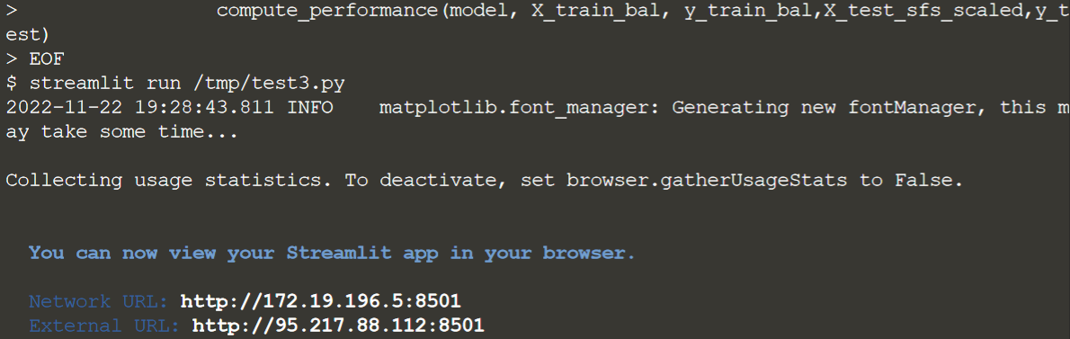
Здесь вы можете увидеть весь скрипт и выполнить его, чтобы получить итоговый вью на дашборде.
cat << EOF > /tmp/test3.py import numpy as np import pandas as pd import matplotlib.pyplot as plt import timeit import warnings warnings.filterwarnings("ignore") import streamlit as st import streamlit.components.v1 as components #Import classification models and metrics from sklearn.linear_model import LogisticRegression from sklearn.neighbors import KNeighborsClassifier from sklearn.svm import SVC from sklearn.ensemble import RandomForestClassifier,ExtraTreesClassifier from sklearn.model_selection import cross_val_score #Import performance metrics, imbalanced rectifiers from sklearn.metrics import confusion_matrix,classification_report,matthews_corrcoef from imblearn.over_sampling import SMOTE from imblearn.under_sampling import NearMiss np.random.seed(42) #for reproducibility since SMOTE and Near Miss use randomizations from pandas_profiling import ProfileReport from streamlit_pandas_profiling import st_profile_report st.title('Claims Prediction') df=pd.read_excel('https://github.com/Stijnvhd/Streamlit_Course/blob/main/3.%20A%20first%20ML%20example/data.xlsx?raw=true', engine='openpyxl',) app_mode = st.sidebar.selectbox('Mode', ['About', 'EDA', 'Analysis']) if app_mode == "About": st.markdown('Claims Prediction Example') st.markdown( """ <style> [data-testid="stSidebar"][aria-expanded="true"] > div:first-child{ width: 350px } [data-testid="stSidebar"][aria-expanded="false"] > div:first-child{ width: 350px margin-left: -350px } </style> """, unsafe_allow_html=True, ) st.markdown('') st.markdown('This dashboard allows you to follow the Claims Prediction Example. It can help you to understand how we can focus on claims and this way develop proper pricing for our products.') elif app_mode == 'EDA': st.sidebar.subheader(' Quick Explore') st.markdown("Tick the box on the side panel to explore the dataset.") if st.sidebar.checkbox('Basic Info'): if st.sidebar.checkbox("Show Columns"): st.subheader('Show Columns List') all_columns = df.columns.to_list() st.write(all_columns) if st.sidebar.checkbox('Statistical Description'): st.subheader('Statistical Data Description') st.write(df.describe()) if st.sidebar.checkbox('Missing Values?'): st.subheader('Missing values') st.write(df.isnull().sum()) elif app_mode == "Analysis": # Print shape and description of the data st.set_option('deprecation.showPyplotGlobalUse', False) if st.sidebar.checkbox('Show DataFrame'): st.write(df.head(100)) st.write('Shape of the dataframe: ',df.shape) st.write('Data decription: \n',df.describe()) # Print valid and fraud transactions fraud=df[df.ClaimNb==1] valid=df[df.ClaimNb==0] outlier_percentage=(df.ClaimNb.value_counts()[1]/df.ClaimNb.value_counts()[0])*100 if st.sidebar.checkbox('Show claim and valid transaction details'): st.write('Claim cases are: %.3f%%'%outlier_percentage) st.write('Claim Cases: ',len(fraud)) st.write('Valid Cases: ',len(valid)) #Obtaining X (features) and y (labels) df=df.drop(['PolicyID'], axis=1) df=df.drop(['Power'], axis=1) df=df.drop(['Brand'], axis=1) df=df.drop(['Gas'], axis=1) df=df.drop(['Region'], axis=1) df=df.dropna() X=df.drop(['ClaimNb'], axis=1) y=df.ClaimNb # Split the data into training and testing sets from sklearn.model_selection import train_test_split size = st.sidebar.slider('Test Set Size', min_value=0.2, max_value=0.4) X_train, X_test, y_train, y_test = train_test_split(X, y, test_size = size, random_state = 42) #Print shape of train and test sets if st.sidebar.checkbox('Show the shape of training and test set features and labels'): st.write('X_train: ',X_train.shape) st.write('y_train: ',y_train.shape) st.write('X_test: ',X_test.shape) st.write('y_test: ',y_test.shape) #Import classification models and metrics from sklearn.linear_model import LogisticRegression from sklearn.neighbors import KNeighborsClassifier from sklearn.svm import SVC from sklearn.ensemble import RandomForestClassifier,ExtraTreesClassifier from sklearn.model_selection import cross_val_score logreg=LogisticRegression() svm=SVC() knn=KNeighborsClassifier() etree=ExtraTreesClassifier(random_state=42) rforest=RandomForestClassifier(random_state=42) features=X_train.columns.tolist() #Feature selection through feature importance @st.cache def feature_sort(model,X_train,y_train): #feature selection mod=model # fit the model mod.fit(X_train, y_train) # get importance imp = mod.feature_importances_ return imp #Classifiers for feature importance clf=['Extra Trees','Random Forest'] mod_feature = st.sidebar.selectbox('Which model for feature importance?', clf) start_time = timeit.default_timer() if mod_feature=='Extra Trees': model=etree importance=feature_sort(model,X_train,y_train) elif mod_feature=='Random Forest': model=rforest importance=feature_sort(model,X_train,y_train) elapsed = timeit.default_timer() - start_time st.write('Execution Time for feature selection: %.2f minutes'%(elapsed/60)) #Plot of feature importance if st.sidebar.checkbox('Show plot of feature importance'): plt.bar([x for x in range(len(importance))], importance) plt.title('Feature Importance') plt.xlabel('Feature (Variable Number)') plt.ylabel('Importance') st.pyplot() feature_imp=list(zip(features,importance)) feature_sort=sorted(feature_imp, key = lambda x: x[1]) n_top_features = st.sidebar.slider('Number of top features', min_value=5, max_value=20) top_features=list(list(zip(*feature_sort[-n_top_features:]))[0]) if st.sidebar.checkbox('Show selected top features'): st.write('Top %d features in order of importance are: %s'%(n_top_features,top_features[::-1])) X_train_sfs=X_train[top_features] X_test_sfs=X_test[top_features] X_train_sfs_scaled=X_train_sfs X_test_sfs_scaled=X_test_sfs smt = SMOTE() nr = NearMiss() def compute_performance(model, X_train, y_train,X_test,y_test): start_time = timeit.default_timer() scores = cross_val_score(model, X_train, y_train, cv=3, scoring='accuracy').mean() 'Accuracy: ',scores model.fit(X_train,y_train) y_pred = model.predict(X_test) cm=confusion_matrix(y_test,y_pred) 'Confusion Matrix: ',cm cr=classification_report(y_test, y_pred) 'Classification Report: ',cr mcc= matthews_corrcoef(y_test, y_pred) 'Matthews Correlation Coefficient: ',mcc elapsed = timeit.default_timer() - start_time 'Execution Time for performance computation: %.2f minutes'%(elapsed/60) #Run different classification models with rectifiers if st.sidebar.checkbox('Run a claims prediction model'): alg=['Extra Trees','Random Forest','k Nearest Neighbor','Support Vector Machine','Logistic Regression'] classifier = st.sidebar.selectbox('Which algorithm?', alg) rectifier=['SMOTE','Near Miss','No Rectifier'] imb_rect = st.sidebar.selectbox('Which imbalanced class rectifier?', rectifier) if classifier=='Logistic Regression': model=logreg if imb_rect=='No Rectifier': compute_performance(model, X_train_sfs_scaled, y_train,X_test_sfs_scaled,y_test) elif imb_rect=='SMOTE': rect=smt st.write('Shape of imbalanced y_train: ',np.bincount(y_train)) X_train_bal, y_train_bal = rect.fit_resample(X_train_sfs_scaled, y_train) st.write('Shape of balanced y_train: ',np.bincount(y_train_bal)) compute_performance(model, X_train_bal, y_train_bal,X_test_sfs_scaled,y_test) elif imb_rect=='Near Miss': rect=nr st.write('Shape of imbalanced y_train: ',np.bincount(y_train)) X_train_bal, y_train_bal = rect.fit_resample(X_train_sfs_scaled, y_train) st.write('Shape of balanced y_train: ',np.bincount(y_train_bal)) compute_performance(model, X_train_bal, y_train_bal,X_test_sfs_scaled,y_test) elif classifier == 'k Nearest Neighbor': model=knn if imb_rect=='No Rectifier': compute_performance(model, X_train_sfs_scaled, y_train,X_test_sfs_scaled,y_test) elif imb_rect=='SMOTE': rect=smt st.write('Shape of imbalanced y_train: ',np.bincount(y_train)) X_train_bal, y_train_bal = rect.fit_resample(X_train_sfs_scaled, y_train) st.write('Shape of balanced y_train: ',np.bincount(y_train_bal)) compute_performance(model, X_train_bal, y_train_bal,X_test_sfs_scaled,y_test) elif imb_rect=='Near Miss': rect=nr st.write('Shape of imbalanced y_train: ',np.bincount(y_train)) X_train_bal, y_train_bal = rect.fit_resample(X_train_sfs_scaled, y_train) st.write('Shape of balanced y_train: ',np.bincount(y_train_bal)) compute_performance(model, X_train_bal, y_train_bal,X_test_sfs_scaled,y_test) elif classifier == 'Support Vector Machine': model=svm if imb_rect=='No Rectifier': compute_performance(model, X_train_sfs_scaled, y_train,X_test_sfs_scaled,y_test) elif imb_rect=='SMOTE': rect=smt st.write('Shape of imbalanced y_train: ',np.bincount(y_train)) X_train_bal, y_train_bal = rect.fit_resample(X_train_sfs_scaled, y_train) st.write('Shape of balanced y_train: ',np.bincount(y_train_bal)) compute_performance(model, X_train_bal, y_train_bal,X_test_sfs_scaled,y_test) elif imb_rect=='Near Miss': rect=nr st.write('Shape of imbalanced y_train: ',np.bincount(y_train)) X_train_bal, y_train_bal = rect.fit_resample(X_train_sfs_scaled, y_train) st.write('Shape of balanced y_train: ',np.bincount(y_train_bal)) compute_performance(model, X_train_bal, y_train_bal,X_test_sfs_scaled,y_test) elif classifier == 'Random Forest': model=rforest if imb_rect=='No Rectifier': compute_performance(model, X_train_sfs_scaled, y_train,X_test_sfs_scaled,y_test) elif imb_rect=='SMOTE': rect=smt st.write('Shape of imbalanced y_train: ',np.bincount(y_train)) X_train_bal, y_train_bal = rect.fit_resample(X_train_sfs_scaled, y_train) st.write('Shape of balanced y_train: ',np.bincount(y_train_bal)) compute_performance(model, X_train_bal, y_train_bal,X_test_sfs_scaled,y_test) elif imb_rect=='Near Miss': rect=nr st.write('Shape of imbalanced y_train: ',np.bincount(y_train)) X_train_bal, y_train_bal = rect.fit_resample(X_train_sfs_scaled, y_train) st.write('Shape of balanced y_train: ',np.bincount(y_train_bal)) compute_performance(model, X_train_bal, y_train_bal,X_test_sfs_scaled,y_test) elif classifier == 'Extra Trees': model=etree if imb_rect=='No Rectifier': compute_performance(model, X_train_sfs_scaled, y_train,X_test_sfs_scaled,y_test) elif imb_rect=='SMOTE': rect=smt st.write('Shape of imbalanced y_train: ',np.bincount(y_train)) X_train_bal, y_train_bal = rect.fit_resample(X_train_sfs_scaled, y_train) st.write('Shape of balanced y_train: ',np.bincount(y_train_bal)) compute_performance(model, X_train_bal, y_train_bal,X_test_sfs_scaled,y_test) elif imb_rect=='Near Miss': rect=nr st.write('Shape of imbalanced y_train: ',np.bincount(y_train)) X_train_bal, y_train_bal = rect.fit_resample(X_train_sfs_scaled, y_train) st.write('Shape of balanced y_train: ',np.bincount(y_train_bal)) compute_performance(model, X_train_bal, y_train_bal,X_test_sfs_scaled,y_test) EOF Прежде чем пытаться запустить приведенный выше код, нажмите Ctrl + C, чтобы остановить запуск текущей панели инструментов в вашем терминале. Затем запустите приведенный ниже фрагмент кода и перезагрузите панель управления, чтобы увидеть изменения!
Вы можете запустить панель управления, выполнив команду streamlit run /tmp/test3.py

Пользуясь случаем, рекомендую посетить открытый онлайн-урок по методам ансамблирования в машинном обучении. На занятии планируется разобрать основные подходы к ансамблированию, которые сегодня используют в ML, изучить устройство наиболее популярных методов ансамблирования (Bagging, Random Forest, Boosting) и применить их сразу на практике. Регистрация доступна по ссылке ниже.
ссылка на оригинал статьи https://habr.com/ru/company/otus/blog/701412/
Добавить комментарий